Discussion

If we used regression tools, there are many models that will fit the curve quite well, for example:
The cubic curve y = 0,000002x³ – 0,0062x² + 2,6884x – 112,75, R² = 0,9993
The quartic curve y = -0,00000001x⁴ + 0,00001x³ – 0,0101x² + 3,2154x – 133,84, R2 = 0,9998
The sinusoidal curve y = -1238,6094 + 1445,1165*cos(0,0025250398x – 0.65004446), r = 0,9984326

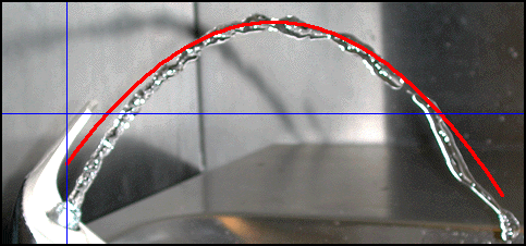
It is important to determine the function type on theoretical or structural grounds! In this case, any particle of water is in fact a projectile, a freefalling body: after projection the only force acting on the particle is gravity! Therefore, the appropriate function is a parabola, as proved in Unit 11.

It is important to realise that our parabola function will not fit the data exactly, for at least two reasons:

• The curve is far from perfect, maybe because the water pressure is uneven. There is some evidence for this on the left side of the curve formed by the squirt. Notice how irregular this part of the curve is.
• Our measurement of positions on the curve in the applet cannot be very accurate, so it is to be expected that our parabola function will not fit the data exactly.

If you used the Excel tools, you would get a fairly reasonable parabola of best fit with approximate formula:
f(x) = -0,0045x² + 2,310x – 92,85

However, you should also be able to do it easier algebraically, by using your knowledge of equations of the parabola. For example, We can use the form f(x) = a(x – p)² + q where (p, q) are the coordinates of the turning point. So try to get a good reading for (p, q), e.g. (250, 204).

Then the equation is f(x) = a(x – 250)² + 204.

To solve for a, we need just more good measurement, say (300, 195), then

Entering this formula as -0.0036*(x - 250)^2 + 204 in the interval [40, 460] in the applet gives a reasonably good fit for the squirt curve, which we can now further improve if we want to: